
Published 2024-01-24.
Last modified 2024-02-11.
Time to read: 21 minutes.
llm collection.
Introduction
The following video is a no-holds-barred, python-code-writing tour-de-force that explains and then implements some of the main concepts used in diffusion LLMs. It is a very dense condensation of knowledge, and the material flies by fast.
You need to have an understanding of probability theory in order to understand the mathematics presented in the video. I provide a quick refresher Quick Review of Probability Theory.
Reading along with a transcript greatly assists comprehension; merely turning on YouTube captions is insufficient to comprehend the verbal firehose that this video subjects you to.
Please understand, I mean this in the nicest way. The speaker, Tushar Kumar, has mastered his subject; however, he is merciless in his relentless recounting of the story.
I found the speaker’s accent occassionally very difficult to understand. Some words just did not come through clearly.
The speaker also says cross when I would say by, as in “this image has dimensions 512x512 pixels”. I was unsure at first if he was referring to a cross product, which is a common operation for vectors, but he seems to always mean by instead.
Use every advantange you can to assimilate the information. This is a course module, not just a video, and although it seems very complete, the material is not presented in a readily digestible manner. That is unfortunate, because all the work had been done in order to do a better presentation.
Transcripts and Annotations
I explained how easy it is to get such a transcript in
OpenAI Whisper.
Just visit the free Face.co/spaces/openai/whisper Whisper Large V3 public instance,
click on the YouTube tab, and paste in the url for the YouTube video:
https://www.youtube.com/watch?v=vu6eKteJWew,
then press the Submit button.
Here is a formatted and annotated version of the transcription, wrapped at 72 columns. A few phrases were not transcribed, and some words were incorrectly transcribed. I present corrected text in the remainder of this article.
In this video, I'll cover the implementation of diffusion models. We'll
create DDPM for now, and in later videos, move to stable diffusion with
text prompts. In this one, we'll be implementing the training and
sampling part for DDPM. For our model, we'll actually implement the
architecture that is used in latest diffusion models, rather than the
one originally used in DDPM. We'll dive deep into the different blocks
in it, before finally putting everything in code, and see results of
training this diffusion model on grayscale and RGB images. I'll cover
the specific math of diffusion models that we need for implementation
very quickly in the next few minutes. But this should only act as a
refresher, so if you're not aware of it and are interested in knowing
it, I would suggest to first see my diffusion math video that's linked
above. The entire diffusion process involves a forward process where we
take an image and create noisier versions of it step by step, by adding
Gaussian noise. After a large number of steps, it becomes equivalent to
a sample of noise from a normal distribution. We do this by applying
this transition function at every timestep t, and beta is a scheduled
noise which we add to the image at t-1 to get the image at t. We saw
that having alpha as 1-beta and computing cumulative products of these
alphas at time t allows us to jump from original image to noisy image at
any timestep t in the forward process. We then have a model learn the
reverse process distribution and because the reverse diffusion process
has the same functional form as the forward process which here is a
Gaussian, we essentially want the model to learn to predict its mean and
variance. After going through a lot of derivation from the initial goal
of optimizing the log likelihood of the observed data, we ended with the
requirement to minimize the KL divergence between the ground truth
renoising distribution conditioned on X0, which we computed as having
this mean and this variance, and the distribution predicted by our
model. We fixed the variance to be exactly same as the target
distribution and rewrite the mean in the same form. After this,
minimizing KL divergence ends up being minimizing square of difference
between the noise predicted and the original noise sample. Our training
method then involves sampling an image, timestep t, and a noise sample
and feeding the model the noisy version of this image at sample timestep
t using this equation. The cumulative product terms needs to be coming
from the noise scheduler, which decides the schedule of noise added as
we move along timesteps. And loss becomes the MSC between the original
noise and whatever the model predicts. For generating images, we just
sample from our learnt reverse distribution, starting from a noise
sample xt from a normal distribution, learned reverse distribution,
starting from a noise sample X from a normal distribution and then
computing the mean using the same formulation, just in terms of X and
noise prediction and variance is same as the ground truth denoising
distribution conditioned on X. Then we get a sample from this reverse
distribution using the reparameterization trick and repeating this gets
us to X. And for X we don't add any noise and simply return the mean.
This was a very quick overview and I had to skim through a lot. For a
detailed version of this, I would encourage you to look at the previous
diffusion video. So for implementation, we saw that we need to do some
computation for the forward and the reverse process. So we will create a
noise scheduler which will do these two things for us. For the forward
process, given an image and a noise sample and timestep t, it will
return the noisy version of this image using the forward equation. And
in order to do this efficiently, it will store the alphas, which is just
1 minus beta, and the cumulative product terms of alpha for all t. The
authors use a linear noise scheduler where they linearly scale beta from
1e-4 to 0.02 with 1000 timesteps between them and we will also do the
same. The second responsibility that this scheduler will do is given in
xt and noise prediction for a model it will give us xt-1 by sampling
from the reverse distribution. it'll give us xt-1 by sampling from the
reverse distribution. For this, it'll compute the mean and variance
according to their respective equations and return a sample from this
distribution using the reparameterization trick. To do this, we also
store 1-alpha t, 1-the cumulative product terms, and its square root.
Obviously, we can compute all of this at runtime as well, but
pre-computing them simplifies the code for the equation a lot. So let's
implement the noise scheduler first. As I mentioned, we'll be creating a
linear noise schedule. After initializing all the parameters from the
arguments of this class, we'll create betas to linearly increase from
start to end such that we have beta t from 0 till the last timestep.
We'll then initialize all the variables that we need for forward and
reverse process The add underscore noise method is our forward process.
So it will take in an image, original noise sample and timestep t. The
images and noise will be of B cross C cross H cross W and timestep will
be a 1D tensor of size b. For the forward process we need the square
root of cumulative product terms for the given timesteps and 1 minus
that and then we reshape them so that they are b cross 1 cross 1 cross
1. Lastly we apply the forward process equation. The second function
will be the guy that takes the image xt and gives us a sample from our
learned reverse distribution. For that we'll have it receive xt and
noise prediction from the model and timestep t as the argument. We'll be
saving the original image prediction x0 for visualizations and get that
using this equation. This can be obtained using the same equation for
forward process that takes from x0 to xt by just rearranging the terms
and using noise prediction instead of the actual noise. Then for
sampling we'll compute the mean and noise is only added for other time
steps. The variance of that is same as the variance of ground truth,
renoising which was this. And lastly we'll sample from a Gaussian
distribution with this mean and variance using the reparameterization
trick. This completes the entire noise scheduler which handles the
forward process of adding noise and the reverse process of sampling
first. Let's now get into the model. For diffusion models we are
actually free to use whatever architecture we want as long as we meet
two requirements. The first being that the shape of the input and output
must be same and the other is some mechanism to fuse in timestep
information. Let's talk about why for a bit. The information of what
timestep we are at is always available to us, whether we are at
training or sampling. And in fact, knowing what timestep we are at
would aid the model in predicting original noise, because we are
providing the information that how much of that input image actually is
noise. So instead of just giving the model an image, we also give the
timeep that we are at. For the model, I'll use unit, which is also what
the authors use, but for the exact specification of the blocks,
activations, normalizations and everything else, I'll mimic the stable
diffusion unit used by Hugging Face in the diffusers pipeline. That's
because I plan to soon create a video on stable diffusion, so that'll
allow me to reuse a lot of code that I'll create now. Actually, even
before going into the unit model, let's first see how the timestep
information is represented. Let's call this the time embedding block
which will take in a 1D tensor of timesteps of size b which is batch
size and give us a t underscore emb underscore dim size representation
for each of those timeeps in the batch. The time embedding block would
first convert the integer timesteps into some vector representation
using an embedding space. That will then be fed to two linear layers
separated by activation to give us our final timestep representation.
For the embedding space, the authors used the sinusoidal position
embedding used in transformers. For activations, everywhere I have used
sigmoid linear units, but you can choose a different For the embedding
space, the authors used the sinusoidal position embedding used in
transformers. For activations, everywhere I have used sigmoid linear
units, but you can choose a different one as well. Okay, now let's get
into the model. As I mentioned, I'll be using UNET just like the
authors, which is essentially this encoder-decoder architecture, where
encoder is a series of downsampling blocks where each block reduces the
size of the input, typically by half, and increases the number of
channels. The output of final downsampling block is passed to layers of
midblock which all work at the same spatial resolution. And after that
we have a series of upsampling blocks. These one by one increase the
spatial size and reduce the number of channels to ultimately match the
input size of the model. The upsampling blocks also fuse in the output
coming from the corresponding downsampling block at the same resolution
via residual skip connections. Most of the diffusion models usually
follow this unit architecture, but differ based on specifications
happening inside the blocks. And as I mentioned, for this video I have
tried to mimic to some extent what's happening inside the stable
diffusion unit from Hugging Face. Let's look closely into the down
block and once we understand that, the rest are pretty easy to follow.
Down blocks of almost all the variations would be a ResNet block
followed by a self-attention block and then a downsample layer. For our
ResNet plus self-attention block, we'll have group norm followed by
activation followed by a convolutional layer. The output of this will
again be passed to a normalization, activation and convolutional layer.
We add a residual connection from the input of first normalization layer
to the output of second convolutional layer. This entire thing is what
will be called as a ResNet block, which you can think of as two
convolutional blocks plus residual connection. This is then followed by
a normalization and a self-attention layer, and again residual
connection. We have multiple such ResNet plus self-attention layers, but
for simplicity our current implementation will only have one layer. The
code on the repo however will be configurable to make as many layers as
desired. We also need to fuse the time information and the way it's done
is that each ResNet block has an activation followed by a linear layer.
And we pass the time embedding representations through them first before
adding to the output of the first convolutional layer. So essentially
this linear layer is projecting the t underscore emb underscore dim
timestep representation to a tensor of same size as the channels in the
convolutional layer's output. That way these two can be added by
replicating this timestep representation across the spatial dimension.
Now that we have seen the details inside the block, to simplify, let's
replace everything within this part as a ResNet block and within this as
a self-attention block. The other two blocks are using the same
components and just slightly different. Let's go back to our previous
illustration of all three blocks. We saw that down block is just
multiple layers of ResNet followed by self-attention. And lastly we have
a down sampling layer. Up block is exactly the same, except that it
first upsamples the input to twice the spatial size, and then
concatenates the down block output of the same spatial resolution across
the channel dimension. Post that, it's the same layers of resnet and
self-attention blocks. The layers of mid block always maintain the input
to the same spatial resolution. The Hugging Face version has first one
ResNet block, and then followed by layers of Self-Attention and ResNet.
So I also went ahead and made the same implementation. And let's not
forget the Timestep information. For each of these ResNet blocks, we
have a Timestep projection layer. This was what we just saw, an
activation followed by a linear layer. The existing timestep
representation goes through these blocks before being added to the
output of first convolution layer of the ResNet block. Let's see how all
of this looks in code. The first thing we'll do is implement the
sinusoidal position embedding code. This function receives B-sized 1D
tensor timesteps, where B is the batch size, and is expected to return B
x T underscore EMB underscore DIMM tensor. We first implement the factor
part, which is everything that the position, which here is the timestep
integer value, will be divided with inside the sine and cosine
functions. This will get us all values from 0 to half of the time
embedding dimension size, half because we will concatenate sine and
cosine. After replicating the timestep values, we get our desired shape
tensor and divide it by the factor that we computed. This is now exactly
the arguments for which we have to call the sine and cosine function.
Again all this method does is convert the integer timestep
representation to embeddings using a fixed embedding space. Now we will
be implementing the down block. But before that, let's quickly take a
peek at what layers we need to implement. So we need layers of resnet
plus self-attention blocks. Resnet will be two norm activation
convolutional layers with residual and self-attention will be norm
followed by self-attention. We also need the time projection layers
which will project the time embedding onto the same dimension as the
number of channels in the output of first convolution feature map. I'll
only implement the block to have one layer for now hence we'll only need
single instances of these. And after ResNet and self-attention, we have
a downsampling. Okay back to coding it. For each downblock, we'll have
these arguments. in underscore channel is the number of channels
expected in input. out underscore channels is the channels we want in
the output of this downblock. Then we have the embedding dimension. I
also add a downsample argument, just so that we have the flexibility to
ignore the downsampling part in the code. Lastly num underscore heads is
the number of heads that our retention block will have. This is our
first convolution block of ResNet. We make the channel conversion from
input to output channels via the first conv layer itself. So after this
everything will have out underscore channels as the number of channels.
Then these are the time projection layers for this ResNet block.
Remember each ResNet block will have one of these and we had seen that
this was just activation followed by a linear layer. The output of this
linear layer should have out underscore channels so that we can do the
addition. This is the second gone block which will be exactly same
except everything operating on out underscore channels as the channel
dimension. And then we add the attention part, the normalization and
multihead attention. The feature dimension for multihead attention will
be same as the number of channels. This residual connection is 1x1
conglare and this ensures that the input to the entire ResNet block can
be added to the output of the last conv layers. And since the input was
in underscore channels, we have to first transform it to out underscore
channels so this just does that. And finally we have the downsample
layer which can also be average pooling but I've used convolution with
stride 2 and if the arguments convey to not downsample then this is just
identity. The forward method will be very simple. We first pass the
input to the first con block and then add the time information and then
after going through the second con block we add the residual but only
after passing through the 1 cross 1 con player. Attention will happen
between all the spatial HxW cells, with out underscore channels being
the feature dimensionality of each of those cells. So the transpose just
ensures that the channel features are the last dimension. And after the
channel dimension has been enriched with self-attention representation,
we do the transpose back and again have the residual connection. If we
would be having multiple layers then we would loop over this entire
thing but since we are only implementing one layer for now, we'll just
call the downsampling convolution after this. Next up is mid block and
again let's revisit the illustration for this. For mid block we'll have
a ResNet block and then layers of self-attention, followed by resnet.
Same as down block, we'll only implement one layer for now. The code for
mid block will have same kind of layers, but we need 2 instances of
every layer that belongs to the resnet block, so let's just one
difference, that is we call the first Resonant Block and and then
self-attention and second ResNet block. Had we implemented multiple
layers, the self-attention and the following ResNet block would have a
loop. Now let's do up block, which will be exactly same as down block
except that instead of down sampling we'll have a up sampling layer.
We'll use conf transpose to do the up sampling for us. In the forward
method, let's first copy everything that we did for down block. Then we
need to make three changes. Add the same spatial resolutions down block
output as argument. Then before ResNet plus self-attention blocks, we'll
upsample the input and concat the corresponding down block output.
Another way to implement this could be to first concat, followed by
resnet and self-attention and then upsample, but I went with this one.
Finally we'll build our unit class. It will receive the channels in
input image as argument. We'll hardcode the down channels and mid
channels for now. The way the code is implemented is that these 4 values
of down channels will essentially be converted into 3 down blocks, each
taking input of channel i dimensions and converting it to output of
channel i plus 1 dimensions. And same for the mid blocks. This is just
the downsample arguments that we are going to pass to the blocks.
Remember our time embedding block had position embedding followed by
linear layers with activation in between. These are those two linear
layers. This is different from the timestep layers which we had for each
ResNet block. This will only be called once in an entire forward pass,
right at the start to get initial timestep representation. We'll also
first have to convert the input to have the same channel dimensions as
the input of first down block and this convolution will just do that for
us. We then create the down blocks, mid blocks and up blocks based on
the number of channels provided. For the last up block, I simply
hardcode the output channel as 16. The output of last up block undergoes
a normalization and convolution to get us to the same number of channels
as the input image. We'll be training on MNIST dataset to the same
number of channels as the input image. We'll be training on MNIST
dataset, so the number of channels in the input image would be one. In
the forward method, we first call the conv underscore in layer, and then
get the timestep representation by calling the sinusoidal position
embedding, followed by our linear layers. Then we just call the down
blocks, and we keep saving the output of down blocks because we need it
as input for the up block. During up block calls, we simply take down
outputs from that list one by one and pass that together with the
current output. And then we call our normalization, activation and
output convolution. Once we pass a 4x1x28x28 input tensor to this, we
get the following output shapes. So you can see because we had
downsampled only twice, our smallest size input to any convolution layer
is 7x7. The code on the repo is much more configurable and creates these
blocks based on whatever configuration is passed and can create multiple
layers as well. We'll look at a sample config file later, but first
let's take a brief look at the dataset, training and sampling code. The
dataset class is very simple, it just takes in the path where the images
are and then stores the filename of all those images in there. Right now
we are building unconditional diffusion model, so we don't really use
the labels. Then we simply load the images and convert it to tensor and
we also scale it from minus one to one, just like the authors, so that
our model consistently sees similarly scaled images as compared to the
random noise. Moving to train underscore DDPM file, where the train
function loads up the config and gets the model, dataset, diffusion and
training configurations from it. We then instantiate the noise
scheduler, dataset and our model. After setting up the optimizer and the
loss functions, we run our training loop. Here we take our image batch,
sample random noise of shape B x 1 x h x w, and sample random timesteps.
The scheduler adds noise to these batch images based on the sample
timesteps, and we then backpropagate based on the loss between noise
prediction by our model and the actual noise that we added. For
sampling, similar to training, we load the config and necessary
parameters, our model and noise scheduler. The sample method then
creates a random noise sample based on number of images requested and
then we go through the timesteps in reverse. For each timestep we get
our model's noise prediction and call the reverse process of scheduler
that we had created with this xt and noise prediction and then it
returns the mean of xt-1 and estimate of the original image. We can
choose to either save one of these to see the progress of sampling. Now
let's also take a look at our config file. This just has the dataset
parameters, which stores our image path. Model params, which stores
parameters necessary to create model like the number of channels, down
channels and so on. Like I had mentioned, we can put in the number of
layers required in each of our down, mid and up blocks. And finally we
specify the training parameters. The unit class in the repo has blocks,
which actually read this config and create model based on whatever
configuration is provided. It does everything similar to what we just
implemented, except that it loops over the number of layers as well. And
I've also added shapes of the output that we would get at each of those
block calls so that it helps a bit in understanding everything. For
training, as I mentioned, I train on MNIST, but in order to see if
everything works for RGB images, I also train on this dataset of texture
images, because I already have it downloaded since my video on
implementing DALI. Here is a sample of images from this dataset. These
are not generated, these are images from the dataset itself. Though the
dataset has 256x256 images, I resized the images to be 28x28, primarily
because I lack two important things for training on larger sized images,
patience and compute, rather cheap compute. For MNIST I train it for
about 20 epochs taking 40 minutes on V100 GPU and for this texture
dataset I train for about 60 epochs taking roughly about 3 hours. And
that gives me these results. Here I am saving the original image
prediction at each timestep. And you can see that because MNIST images
are all similar looking, the model pretty quickly gets a decent original
image prediction at each timestep and you can see that because MNIST
images are all similar looking the model pretty quickly gets a decent
original image prediction whereas for the textured data set it doesn't
till about last 200-300 timesteps but by the end of all the steps we
get decent results for both the data sets you can obviously train it on
a larger size data set though probably you would have to maybe increase
the channels and maybe train for longer epochs to get nice results. So
that's all that I wanted to cover for implementing DDPM. We went through
scheduler implementation, unit implementation and saw how everything
comes together in the training and sampling code. Hopefully it gave you
a better understanding of diffusion models. And thank you so much for
watching this video and if you are liking the content and getting
benefit from it, do subscribe the channel. See you in the next video.
The code is on GitHub. This article applies the transcript to the code, a piece at a time. The GitHub repository has instructions for running the code. My purpose is to understand the code by walking through it, not running it.
Original Paper and GitHub Repo
The original paper, Denoising Diffusion Probabilistic Models by Ho, Jain and Abbeel,
can be downloaded as a PDF;
it is referenced as DDPM.pdf in the remainder of this article.
I also looked at the corresponding GitHub repository.
The two GitHub projects are both written in Python. The original project did not use classes, whereas the newer project does. The use of classes makes the code easier to read and to work with.
Please refer to my Large Language Model Notes if you encouter an unfamiliar term.
I have written about how I used MathLive to format the mathematical expressions in this article.
Formatted and Annotated Transcription
From Denoising Diffusion Probabilistic Models Code | DDPM Pytorch Implementation, by Tushar Kumar.
Introduction
In this video, I'll cover the implementation of diffusion models. We'll create DDPM (Denoising Diffusion Probabilistic Models) for now, and in later videos, move to stable diffusion with text prompts. In this one, we'll be implementing the training and sampling part for DDPM.
For our model, we'll actually implement the architecture that is used in latest diffusion models, rather than the one originally used in DDPM. We'll dive deep into the different blocks in it, before finally putting everything in code, and see results of training this diffusion model on grayscale and RGB images.
I'll cover the specific math of diffusion models that we need for implementation very quickly in the next few minutes. But this should only act as a refresher, so if you're not aware of it and are interested in knowing it, I would suggest to first see my diffusion math video that's linked above.
Math Refresher
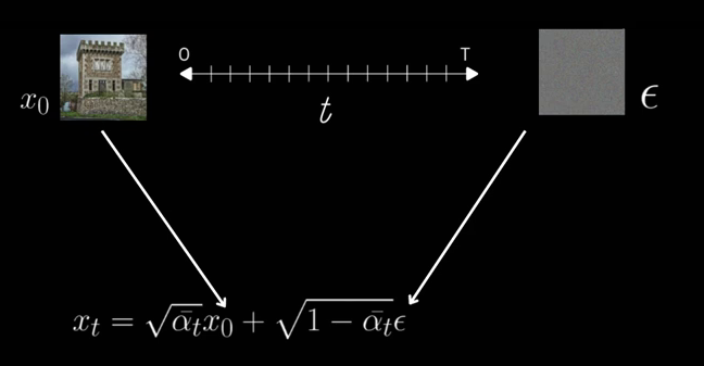
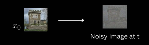
The entire diffusion process involves a forward process where we take an image and create noisier versions of it step by step, by adding Gaussian noise. After a large number of steps, it becomes equivalent to a sample of noise from a normal distribution.

We do this by applying this transition function at every timestep t, and \beta is a scheduled noise which we add to the image at t-1 to get the image at t.
\displaystyle q(x_t|x_{t-1}) \sim \mathcal{N}(x_t; \sqrt{1-\beta_t}x_{t-1}, \beta_t\Pi)
This is the forward transition function \displaystyle q(x_t|x_{t-1}) for the model, which is a Quick Review of Probability Theory.
We saw that having
\alpha_t=1-{\beta_t}
Precomputing \alpha_t values provides convenience and computational efficiency. The scheduled Gaussian noise \beta_t can only have values ranging from 0 to 1, so \alpha_t will have values varying from 1 to 0.
and computing cumulative products of these \alphas at time t
\displaystyle\overline{\alpha}_t =\prod_{i = 1}^{t}\alpha_i
Precomputed \overline{\alpha}_t values, representing the cumulative products of \alpha_t.
allows us to jump from original image to noisy image at any timestep t in the forward process.
\displaystyle x_t = \sqrt{\overline{\alpha}_t}x_0 + \sqrt{1- \overline{\alpha}_t}\epsilon
Obtaining the noisy image x_t using the forward process
We then have a model learn the reverse process distribution

and because the reverse diffusion process has the same functional form as the forward process, which here is a Gaussian.
q(x_{t-1}|x_{t}) \sim \mathcal{N}\Big(x_{t-1}; \mu_q, \sum_q\Big)
We essentially want the model to learn to predict its mean and variance.
\displaystyle p_0(x_{t-1}|x_{t}) \longrightarrow \mathcal{N}\Big(x_{t-1}; \mu_\theta, \textstyle\sum_{\theta}\Big)
After going through a lot of derivation from the initial goal of optimizing the log likelihood of the observed data,
\displaystyle \log p(x_0) = \log \int p(x_{0:T})dx_{1:T}
we ended with the requirement to minimize the
KL divergence
between the ground truth renoising distribution conditioned on X0.
q(x_{t-1}|x_{t}, x_{0})
We computed this as having this mean
\displaystyle \mu_q = \Big( \frac{(1-\overline{\alpha}_{t-1}) \sqrt{\alpha_t} }{ 1-\overline{\alpha}_t } + \frac{1-\alpha_t}{(\sqrt{\alpha_t})(1-\overline{\alpha}_t)} \Big)x_t - \frac{ (1-\alpha_t)(\sqrt{1-\overline{\alpha}_t)} }{ (1-\overline{\alpha}_t)\sqrt{\alpha_t} }\epsilon
and this variance,
\textstyle\sum_{}_q(t) = \displaystyle \frac{ (1-\alpha_t)(1-\overline{\alpha}_{t-1}) }{ (1-\overline{\alpha}_t) }\Pi
and the distribution predicted by our model.
\displaystyle p_\theta(x_{t-1}|x_{t})
We fixed the variance to be exactly same as the target distribution. Seems like the video mixes up this variance and mean.
and rewrite the mean in the same form.
\displaystyle \Big( \frac{(1-\overline{\alpha}_{t-1}) \sqrt{\alpha_t} }{ 1-\overline{\alpha}_t } + \frac{1-\alpha_t}{(\sqrt{\alpha_t})(1-\overline{\alpha}_t)} \Big)x_t - \frac{ (1-\alpha_t)(\sqrt{1-\overline{\alpha}_t)} }{ (1-\overline{\alpha}_t)\sqrt{\alpha_t} }\epsilon_\theta
After this, minimizing KL divergence ends up being minimizing the square of the difference between the noise predicted and the original noise sample.
The author wrote the equation this way:
\displaystyle \left\Vert\Big(\epsilon_\theta - \epsilon\Big)_2^2\right\Vert
But I think the following may be what he meant:
\displaystyle \Big\Vert\epsilon_\theta - \epsilon\Big\Vert_2^2
Alon Amit has a good explanation of the notation used in my formula above: the subscript2 means “L2 norm”, and the superscript is simply squaring. The L2 norm is the usual Euclidean norm (square root of the sum of squares), and it can be attached as a subscript or superscript to the double bar brackets. If you’re also squaring things, it’s reasonable to keep it at the bottom.
However the following would be a more common of writing the formula:
\displaystyle \Big\Vert\epsilon_\theta - \epsilon\Big\Vert
Training

Our training method then involves sampling an image, timestep t, and a noise sample

and feeding the model (as shown previously)
\displaystyle x_t = \sqrt{\overline{\alpha}_t}x_0 + \sqrt{1- \overline{\alpha}_t}\epsilon
the noisy version of the image at sample timestep t using this equation.
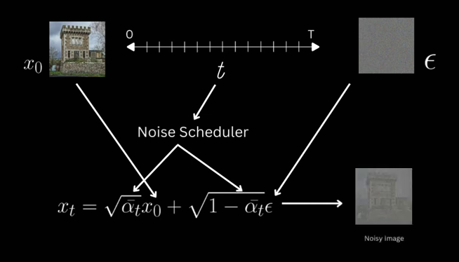
The cumulative product terms needs to be coming from the noise scheduler, which decides the schedule of noise added as we move along timesteps.
And loss becomes the MSE (Mean Squared Error) between the original noise and whatever the model predicts.
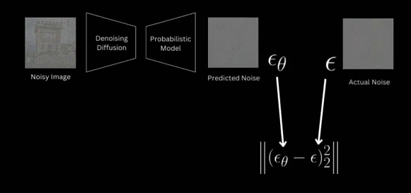
Image Generation

For generating images, we just sample from our learnt reverse distribution,
starting from a noise sample xt from a normal distribution,
\displaystyle p_\theta(x_{t-1}|x_t) \longrightarrow \mathcal{N}\Big(x_{t-1}; \mu_\theta(x_{t}), \frac{ (1 - \alpha_t)(1 - \overline\alpha_{t-1}) }{ 1 - \overline\alpha_t }\Pi\Big)
and then computing the mean using the same formulation, just in terms of x_t
\displaystyle \mu_\theta = \frac{x_t}{\sqrt{\alpha_t}} - \frac{ (1-\alpha_t)(\sqrt{1-\overline{\alpha}_t)} }{ (1-\overline{\alpha}_t)\sqrt{\alpha_t} }\epsilon_\theta

and noise prediction and variance is same as the ground truth denoising distribution conditioned on x0 (which we saw earlier).
\textstyle\sum_{}_q(t) = \displaystyle \frac{ (1-\alpha_t)(1-\overline{\alpha}_{t-1}) }{ (1-\overline{\alpha}_t) }\Pi
Then we get a sample from this reverse distribution using the reparameterization trick:

\displaystyle \mu_\theta + \sigma_{t}z \rightarrow x__{T-1}
and repeating this gets us to x_0.
\displaystyle \class{rotate270}{\text{Repeat until t=1}}\left[\begin{aligned} \\ &\mu_\theta = \frac{x_t}{\sqrt{\alpha_t}} - \frac{(1-\alpha_t)(\sqrt{1-\overline\alpha_t})}{(1-\overline\alpha_t)\sqrt{\alpha_t}}\epsilon_\theta \\ &\mu_\theta + \sigma_{t}z \longrightarrow x_{T-1} \\ \end{aligned}
And for x we don’t add any noise and simply return the mean.
\displaystyle \class{rotate270}{\text{Repeat until t=1}}\left[\begin{aligned} \\ &\mu_\theta = \frac{x_t}{\sqrt{\alpha_t}} - \frac{(1-\alpha_t)(\sqrt{1-\overline\alpha_t})}{(1-\overline\alpha_t)\sqrt{\alpha_t}}\epsilon_\theta \\ &\mu_\theta \longrightarrow x_{T-1} \\ \end{aligned}
This was a very quick overview and I had to skim through a lot. For a detailed version of this, I would encourage you to look at the previous diffusion video.
Implementation
Noise Scheduler
So for implementation, we saw that we need to do some computation for the forward and the reverse process. So we will create a noise scheduler which will do these two things for us.
For the forward process, given an image and a noise sample and timestep t, it will return the noisy version of this image using the forward equation.
\displaystyle x_0, t, \epsilon \longrightarrow x_t = \sqrt{\overline\alpha_t}x_0 + \sqrt{1-\overline\alpha_t}\epsilon
And in order to do this efficiently, it will store the \alphas, which as we have already seen is just 1-\beta,
\alpha_t=1-{\beta_t}
and the cumulative product terms of \alpha for all t, as we have already seen.
\displaystyle\overline{\alpha}_t =\prod_{i = 1}^{t}\alpha_i
The authors use a linear noise scheduler where they linearly scale \beta from 1e-4 to 0.02, with 1000 timesteps between them and we will also do the same.
The second responsibility that this scheduler will do is given in x_t and noise prediction for a model it will give us x_t-1 by sampling from the reverse distribution. It’ll give us x_t-1 by sampling from the reverse distribution. For this, it’ll compute the mean and variance according to their respective equations and return a sample from this distribution using the reparameterization trick.
To do this, we also store 1-\alpha t, 1- the cumulative product terms, and its square root. Obviously, we can compute all of this at runtime as well, but pre-computing them simplifies the code for the equation a lot.
Noise Scheduler Pytorch Code for DDPM
So let’s implement the noise scheduler first. As I mentioned, we’ll be creating a linear noise schedule. After initializing all the parameters from the arguments of this class, we’ll create βs to linearly increase from start to end such that we have \beta_t from 0 till the last timestep.
We’ll then initialize all the variables that we need for forward and reverse process.
The add_noise method is our forward process.
So it will take in an image, original noise sample and timestep t.
The images and noise will be of B \times C \times H \times W
and timestep will be a 1D tensor of size b.
For the forward process we need the square root of cumulative product terms for the given timesteps and
1 minus that and then we reshape them so that they are b \times 1 \times 1 \times 1.
The Forward Equation
Lastly, we apply the forward process equation.
The second function will be the guy that takes the image xt and gives us a sample from our learned reverse distribution.
For that, we’ll have it receive xt and noise prediction from the model and timestep t as the argument.
We’ll be saving the original image prediction x0 for visualizations and get that using this equation.
This can be obtained using the same equation for forward process that takes from x0 to xT by just rearranging the terms
and using noise prediction instead of the actual noise.
Then for sampling we’ll compute the mean and noise is only added for other timesteps.
The variance of that is same as the variance of ground truth, renoising which was this.
And lastly we’ll sample from a Gaussian distribution with this mean and variance using the reparameterization trick. This completes the entire noise scheduler which handles the forward process of adding noise and the reverse process of sampling first.
Denoising Diffusion Probabilistic Models Architecture
Let’s now get into the model. For diffusion models we are actually free to use whatever architecture we want as long as we meet two requirements. The first being that the shape of the input and output must be same and the other is some mechanism to fuse in timestep information. Let’s talk about why for a bit.
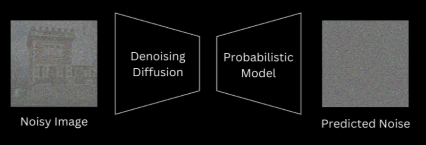
The information of what timestep we are at is always available to us, whether we are at training or sampling. And in fact, knowing what timestep we are at would aid the model in predicting original noise, because we are providing the information that how much of that input image actually is noise.
So instead of just giving the model an image, we also give the timestep that we are at. For the model, I’ll use unit, which is also what the authors use, but for the exact specification of the blocks, activations, normalizations and everything else, I’ll mimic the stable diffusion unit used by Hugging Face in the diffusers pipeline. That’s because I plan to soon create a video on stable diffusion, so that’ll allow me to reuse a lot of code that I’ll create now.
Time embedding Block for DDPM Implementation
Actually, even before going into the unit model, let’s first see how the timestep information is represented.
Let’s call this the time embedding block which will take in a 1D tensor of timesteps of size
t(B,) which is batch size and
give us a t_emb_dim size representation for each of those timesteps in the batch.
The time embedding block would first convert the integer timesteps into some vector representation using an embedding space.
That will then be fed to two linear layers separated by activation to give us our final timestep representation.
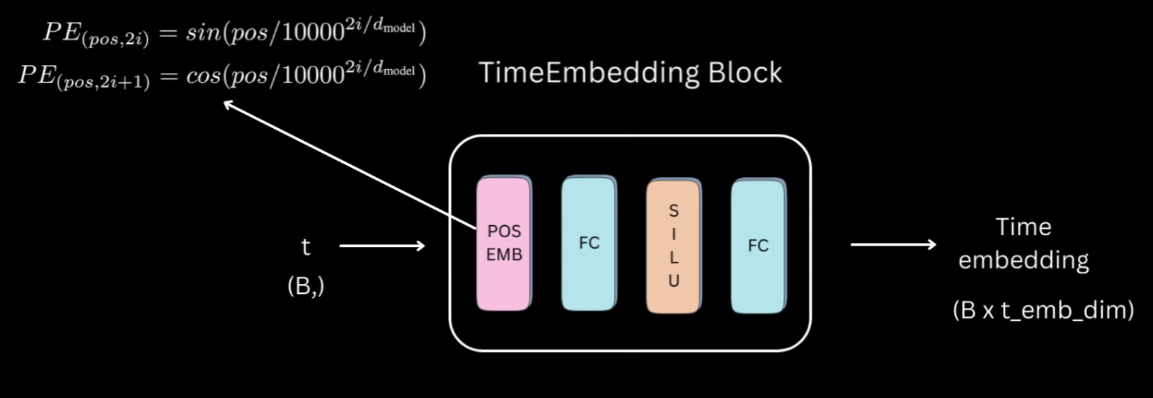
For the embedding space, the authors used the sinusoidal position embedding used in transformers. For activations, everywhere I have used sigmoid linear units, but you can choose a different one as well.
Overview of Unet Architecture for DDPM
Okay, now let’s get into the model. As I mentioned, I’ll be using U-Net just like the authors, which is essentially this encoder-decoder architecture, where encoder is a series of down-sampling blocks where each block reduces the size of the input, typically by half, and increases the number of channels. The output of final down-sampling block is passed to layers of mid-block which all work at the same spatial resolution. And after that we have a series of up-sampling blocks.
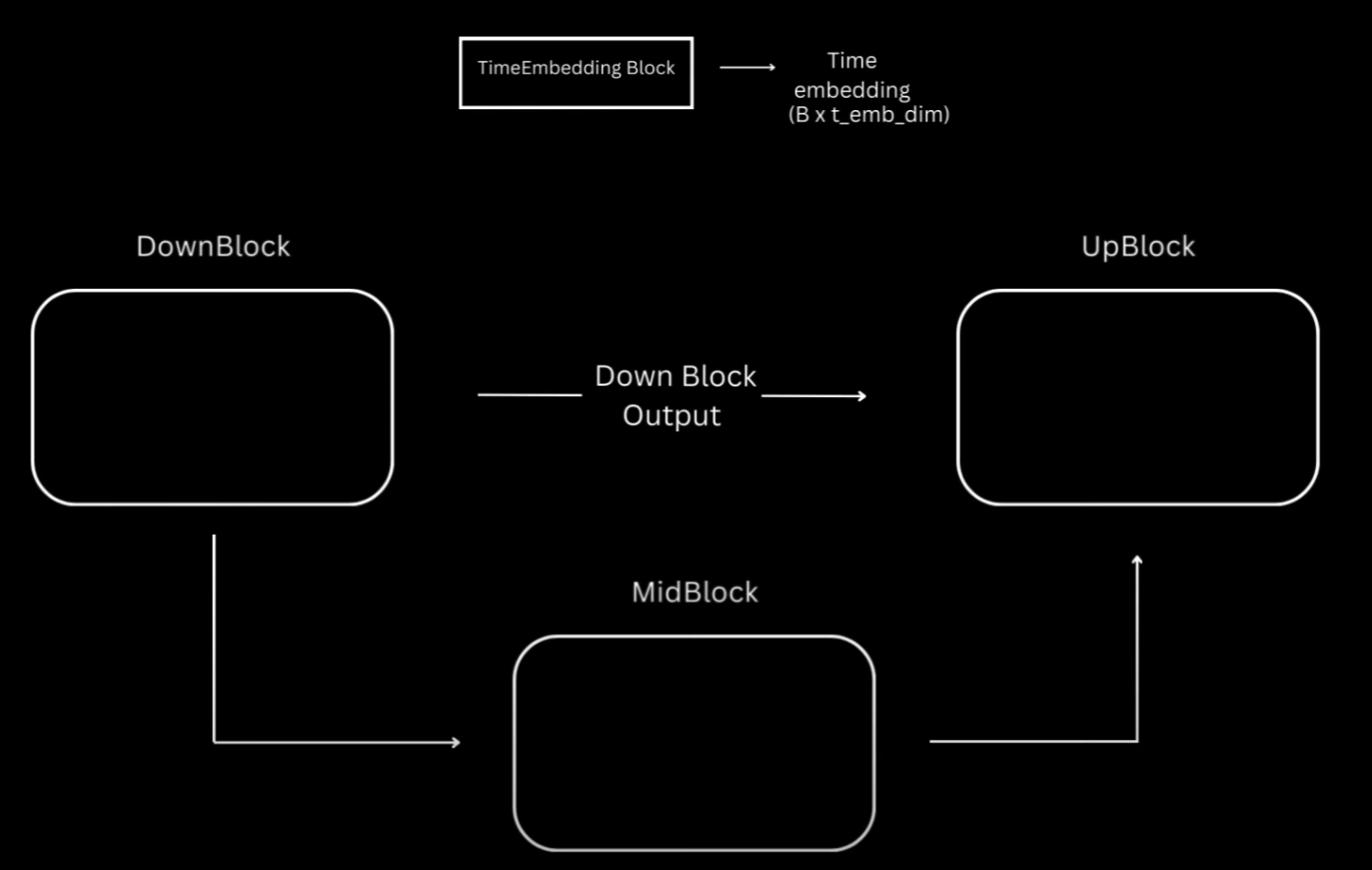
These one by one increase the spatial size and reduce the number of channels to ultimately match the input size of the model. The up-sampling blocks also fuse in the output coming from the corresponding down-sampling block at the same resolution via residual skip connections.
Most of the diffusion models usually follow this unit architecture, but differ based on specifications happening inside the blocks. And as I mentioned, for this video I have tried to mimic to some extent what’s happening inside the stable diffusion unit from Hugging Face.
Downblock of DDPM Unet
Let’s look closely into the down block and once we understand that, the rest are pretty easy to follow. Down blocks of almost all the variations would be a ResNet block, followed by a self-attention block and then a down-sample layer.
For our ResNet + Self Attention block, we’ll have group norm, followed by activation, followed by a convolutional layer. The output of this will again be passed to a normalization, activation and convolutional layer. We add a residual connection from the input of first normalization layer to the output of second convolutional layer. This entire thing is what will be called as a ResNet block, which you can think of as two convolutional blocks plus residual connection.
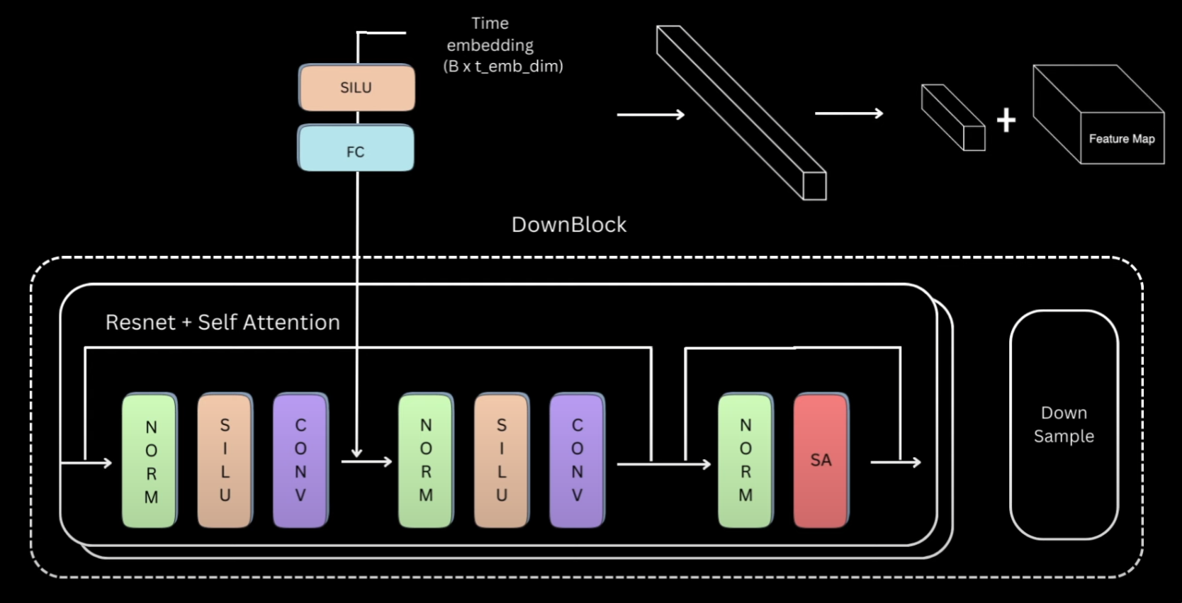
This is then followed by a normalization and a self-attention layer, and again residual connection. We have multiple such ResNet plus self-attention layers, but for simplicity our current implementation will only have one layer. The code on the repository however will be configurable to make as many layers as desired. We also need to fuse the time information and the way it’s done is that each ResNet block has an activation followed by a linear layer.
And we pass the time embedding representations through them first before adding to the output of the first convolutional layer.
So essentially this linear layer is projecting the t_emb_dim timestep representation to a tensor
of same size as the channels in the convolutional layer’s output.
That way these two can be added by replicating this timestep representation across the spatial dimension.
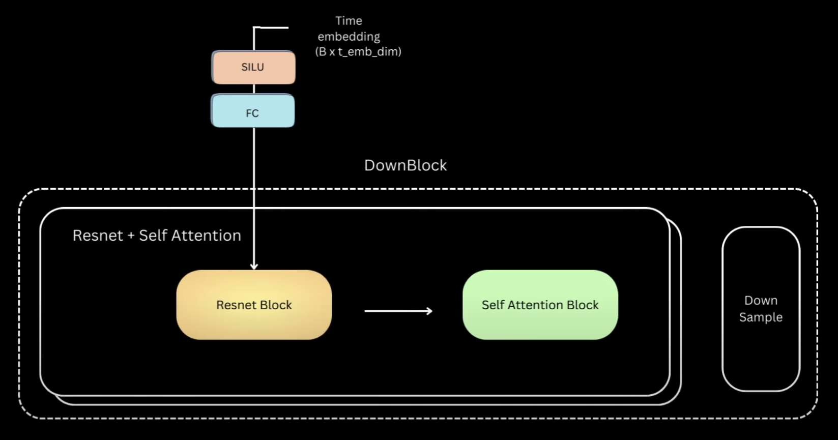
Now that we have seen the details inside the block, to simplify, let’s replace everything within this part as a ResNet block and within this as a self-attention block. The other two blocks are using the same components and just slightly different.
Code for Positional Embedding in DDPM in Pytorch
Let’s go back to our previous illustration of all three blocks. We saw that down block is just multiple layers of ResNet followed by self-attention. And lastly we have a down sampling layer.
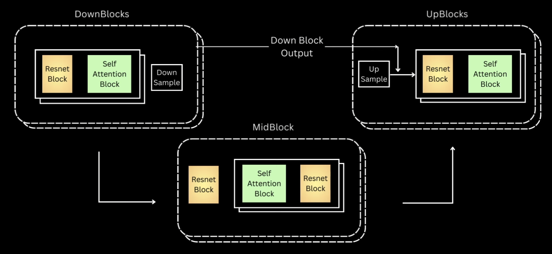
Up block is exactly the same, except that it first upsamples the input to twice the spatial size, and then concatenates the down block output of the same spatial resolution across the channel dimension. Post that, it’s the same layers of resnet and self-attention blocks. The layers of mid block always maintain the input to the same spatial resolution. The Hugging Face version has first one ResNet block, and then followed by layers of Self-Attention and ResNet.
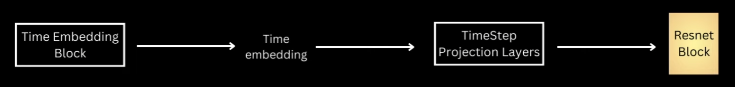
So I also went ahead and made the same implementation. And let’s not forget the Timestep information. For each of these ResNet blocks, we have a Timestep projection layer. This was what we just saw, an activation followed by a linear layer. The existing timestep representation goes through these blocks before being added to the output of first convolution layer of the ResNet block.
Let’s see how all of this looks in code.
Midblock and Upblock for DDPM Unet
The first thing we’ll do is implement the sinusoidal position embedding code. This function receives B-sized 1D tensor timesteps, where B is the batch size, and is expected to return B x T underscore EMB underscore DIMM tensor. We first implement the factor part, which is everything that the position, which here is the timestep integer value, will be divided with inside the sine and cosine functions.
This will get us all values from 0 to half of the time embedding dimension size, half because we will concatenate sine and cosine. After replicating the timestep values, we get our desired shape tensor and divide it by the factor that we computed. This is now exactly the arguments for which we have to call the sine and cosine function.
import torch
import torch.nn as nn

def get_time_embedding(time_steps, temb_dim):
    r"""
    Convert time steps tensor into an embedding using the
    sinusoidal time embedding formula
    :param time_steps: 1D tensor of length batch size
    :param temb_dim: Dimension of the embedding
    :return: BxD embedding representation of B time steps
    """
    assert temb_dim % 2 == 0, "time embedding dimension must be divisible by 2"

    factor = 10000 ** ((torch.arange(
        start=0, end=temb_dim // 2, dtype=torch.float32, device=time_steps.device) / (temb_dim // 2))
    )

    t_emb = time_steps[:, None].repeat(1, temb_dim // 2) / factor
    t_emb = torch.cat([torch.sin(t_emb), torch.cos(t_emb)], dim=-1)
    return t_emb
Again all this method does is convert the integer timestep representation to embeddings using a fixed embedding space. Now we will be implementing the down block.
But before that, let’s quickly take a peek at what layers we need to implement. So we need layers of resnet plus self-attention blocks. Resnet will be two norm activation convolutional layers with residual and self-attention will be norm followed by self-attention. We also need the time projection layers which will project the time embedding onto the same dimension as the number of channels in the output of first convolution feature map.
I’ll only implement the block to have one layer for now hence we’ll only need single instances of these. And after ResNet and self-attention, we have a downsampling. Okay back to coding it.
Code for Downblock in DDPM Unet
For each downblock, we’ll have these arguments in underscore channel is the number of channels expected in input. out underscore channels is the channels we want in the output of this downblock. Then we have the embedding dimension. I also add a downsample argument, just so that we have the flexibility to ignore the downsampling part in the code.
class DownBlock(nn.Module):
    r"""
    Down conv block with attention.
    Sequence of following block
    1. Resnet block with time embedding
    2. Attention block
    3. Downsample using 2x2 average pooling
    """
    def __init__(self, in_channels, out_channels, t_emb_dim,
                 down_sample=True, num_heads=4, num_layers=1):
        super().__init__()
        self.num_layers = num_layers
        self.down_sample = down_sample
        self.resnet_conv_first = nn.ModuleList(
            [
                nn.Sequential(
                    nn.GroupNorm(8, in_channels if i == 0 else out_channels),
                    nn.SiLU(),
                    nn.Conv2d(in_channels if i == 0 else out_channels, out_channels,
                              kernel_size=3, stride=1, padding=1),
                )
                for i in range(num_layers)
            ]
        )
        self.t_emb_layers = nn.ModuleList([
            nn.Sequential(
                nn.SiLU(),
                nn.Linear(t_emb_dim, out_channels)
            )
            for _ in range(num_layers)
        ])
        self.resnet_conv_second = nn.ModuleList(
            [
                nn.Sequential(
                    nn.GroupNorm(8, out_channels),
                    nn.SiLU(),
                    nn.Conv2d(out_channels, out_channels,
                              kernel_size=3, stride=1, padding=1),
                )
                for _ in range(num_layers)
            ]
        )
        self.attention_norms = nn.ModuleList(
            [nn.GroupNorm(8, out_channels)
             for _ in range(num_layers)]
        )

        self.attentions = nn.ModuleList(
            [nn.MultiheadAttention(out_channels, num_heads, batch_first=True)
             for _ in range(num_layers)]
        )
        self.residual_input_conv = nn.ModuleList(
            [
                nn.Conv2d(in_channels if i == 0 else out_channels, out_channels, kernel_size=1)
                for i in range(num_layers)
            ]
        )
        self.down_sample_conv = nn.Conv2d(out_channels, out_channels,
                                          4, 2, 1) if self.down_sample else nn.Identity()
Lastly num_heads is the number of heads that our retention block will have.
This is our first convolution block of ResNet.
We make the channel conversion from input to output channels via the first conv layer itself.
So after this everything will have out underscore channels as the number of channels.
Then these are the time projection layers for this ResNet block.
Remember each ResNet block will have one of these and we had seen that this was just activation followed by a linear layer. The output of this linear layer should have out underscore channels so that we can do the addition. This is the second gone block which will be exactly same except everything operating on out underscore channels as the channel dimension.
And then we add the attention part, the normalization and multihead attention. The feature dimension for multihead attention will be same as the number of channels. This residual connection is 1x1 conglare and this ensures that the input to the entire ResNet block can be added to the output of the last conv layers. And since the input was in underscore channels, we have to first transform it to out underscore channels so this just does that. And finally we have the downsample layer which can also be average pooling but I’ve used convolution with stride 2 and if the arguments convey to not downsample then this is just identity.
The forward method will be very simple.
def forward(self, x, t_emb):
    out = x
    for i in range(self.num_layers):
        # Resnet block of Unet
        resnet_input = out
        out = self.resnet_conv_first[i](out)
        out = out + self.t_emb_layers[i](t_emb)[:, :, None, None]
        out = self.resnet_conv_second[i](out)
        out = out + self.residual_input_conv[i](resnet_input)

        # Attention block of Unet
        batch_size, channels, h, w = out.shape
        in_attn = out.reshape(batch_size, channels, h * w)
        in_attn = self.attention_norms[i](in_attn)
        in_attn = in_attn.transpose(1, 2)
        out_attn, _ = self.attentions[i](in_attn, in_attn, in_attn)
        out_attn = out_attn.transpose(1, 2).reshape(batch_size, channels, h, w)
        out = out + out_attn

    out = self.down_sample_conv(out)
    return out
We first pass the input to the first conv block and then add the time information and then after going through the
second conv block we add the residual but only after passing through the 1 x 1 conv layer.
Attention will happen between all the spatial HxW cells, with out_channels being the feature dimensionality of each of those cells.
So the transpose just ensures that the channel features are the last dimension. And after the channel dimension has been enriched with self-attention representation, we do the transpose back and again have the residual connection.
If we would be having multiple layers then we would loop over this entire thing but since we are only implementing one layer for now, we’ll just call the downsampling convolution after this.
Code for Mid and Upblock in DDPM Unet
Next step is midblock and again let’s revisit the illustration for this.
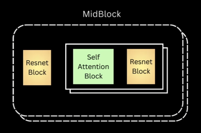
For midblock we’ll have a ResNet block and then layers of self-attention, followed by ResNet. Same as down block, we’ll only implement one layer for now.
class MidBlock(nn.Module):
    r"""
    Mid conv block with attention.
    Sequence of following blocks
    1. Resnet block with time embedding
    2. Attention block
    3. Resnet block with time embedding
    """
    def __init__(self, in_channels, out_channels, t_emb_dim, num_heads=4, num_layers=1):
        super().__init__()
        self.num_layers = num_layers
        self.resnet_conv_first = nn.ModuleList(
            [
                nn.Sequential(
                    nn.GroupNorm(8, in_channels if i == 0 else out_channels),
                    nn.SiLU(),
                    nn.Conv2d(in_channels if i == 0 else out_channels, out_channels, kernel_size=3, stride=1,
                              padding=1),
                )
                for i in range(num_layers+1)
            ]
        )
        self.t_emb_layers = nn.ModuleList([
            nn.Sequential(
                nn.SiLU(),
                nn.Linear(t_emb_dim, out_channels)
            )
            for _ in range(num_layers + 1)
        ])
        self.resnet_conv_second = nn.ModuleList(
            [
                nn.Sequential(
                    nn.GroupNorm(8, out_channels),
                    nn.SiLU(),
                    nn.Conv2d(out_channels, out_channels, kernel_size=3, stride=1, padding=1),
                )
                for _ in range(num_layers+1)
            ]
        )
        self.attention_norms = nn.ModuleList(
            [nn.GroupNorm(8, out_channels)
                for _ in range(num_layers)]
        )
        self.attentions = nn.ModuleList(
            [nn.MultiheadAttention(out_channels, num_heads, batch_first=True)
                for _ in range(num_layers)]
        )
        self.residual_input_conv = nn.ModuleList(
            [
                nn.Conv2d(in_channels if i == 0 else out_channels, out_channels, kernel_size=1)
                for i in range(num_layers+1)
            ]
        )
The code for midblock will have same kind of layers, but we need 2 instances of every layer that belongs to the ResNet block, so let’s just put all of that in.
The forward method will just have one difference, that is we call the first ResNet block, and then self-attention, and then second ResNet block.
def forward(self, x, t_emb):
    out = x

    # First resnet block
    resnet_input = out
    out = self.resnet_conv_first[0](out)
    out = out + self.t_emb_layers[0](t_emb)[:, :, None, None]
    out = self.resnet_conv_second[0](out)
    out = out + self.residual_input_conv[0](resnet_input)

    for i in range(self.num_layers):
        # Attention Block
        batch_size, channels, h, w = out.shape
        in_attn = out.reshape(batch_size, channels, h * w)
        in_attn = self.attention_norms[i](in_attn)
        in_attn = in_attn.transpose(1, 2)
        out_attn, _ = self.attentions[i](in_attn, in_attn, in_attn)
        out_attn = out_attn.transpose(1, 2).reshape(batch_size, channels, h, w)
        out = out + out_attn

        # Resnet Block
        resnet_input = out
        out = self.resnet_conv_first[i+1](out)
        out = out + self.t_emb_layers[i+1](t_emb)[:, :, None, None]
        out = self.resnet_conv_second[i+1](out)
        out = out + self.residual_input_conv[i+1](resnet_input)
    return out
Had we implemented multiple layers, the self-attention and the following ResNet block would have a loop.
Now let’s do up-block, which will be exactly same as down-block except that instead of downsampling we’ll have an upsampling layer.
We’ll use ConvTranspose2d to do the upsampling for us.
class UpBlock(nn.Module):
    r"""
    Up conv block with attention.
    Sequence of following blocks
    1. Upsample
    1. Concatenate Down block output
    2. Resnet block with time embedding
    3. Attention Block
    """
    def __init__(self, in_channels, out_channels, t_emb_dim, up_sample=True, num_heads=4, num_layers=1):
        super().__init__()
        self.num_layers = num_layers
        self.up_sample = up_sample
        self.resnet_conv_first = nn.ModuleList(
            [
                nn.Sequential(
                    nn.GroupNorm(8, in_channels if i == 0 else out_channels),
                    nn.SiLU(),
                    nn.Conv2d(in_channels if i == 0 else out_channels, out_channels, kernel_size=3, stride=1,
                              padding=1),
                )
                for i in range(num_layers)
            ]
        )
        self.t_emb_layers = nn.ModuleList([
            nn.Sequential(
                nn.SiLU(),
                nn.Linear(t_emb_dim, out_channels)
            )
            for _ in range(num_layers)
        ])
        self.resnet_conv_second = nn.ModuleList(
            [
                nn.Sequential(
                    nn.GroupNorm(8, out_channels),
                    nn.SiLU(),
                    nn.Conv2d(out_channels, out_channels, kernel_size=3, stride=1, padding=1),
                )
                for _ in range(num_layers)
            ]
        )
        self.attention_norms = nn.ModuleList(
            [
                nn.GroupNorm(8, out_channels)
                for _ in range(num_layers)
            ]
        )
        self.attentions = nn.ModuleList(
            [
                nn.MultiheadAttention(out_channels, num_heads, batch_first=True)
                for _ in range(num_layers)
            ]
        )
        self.residual_input_conv = nn.ModuleList(
            [
                nn.Conv2d(in_channels if i == 0 else out_channels, out_channels, kernel_size=1)
                for i in range(num_layers)
            ]
        )
        self.up_sample_conv = nn.ConvTranspose2d(in_channels // 2, in_channels // 2,
                                                 4, 2, 1) \
            if self.up_sample else nn.Identity()
In the forward method, let’s first copy everything that we did for down-block. Then we need to make three changes. Add the same spatial resolutions down-block output as argument. Then before ResNet plus self-attention blocks, we’ll upsample the input and concat the corresponding down block output.
def forward(self, x, out_down, t_emb):
    x = self.up_sample_conv(x)
    x = torch.cat([x, out_down], dim=1)

    out = x
    for i in range(self.num_layers):
        resnet_input = out
        out = self.resnet_conv_first[i](out)
        out = out + self.t_emb_layers[i](t_emb)[:, :, None, None]
        out = self.resnet_conv_second[i](out)
        out = out + self.residual_input_conv[i](resnet_input)

        batch_size, channels, h, w = out.shape
        in_attn = out.reshape(batch_size, channels, h * w)
        in_attn = self.attention_norms[i](in_attn)
        in_attn = in_attn.transpose(1, 2)
        out_attn, _ = self.attentions[i](in_attn, in_attn, in_attn)
        out_attn = out_attn.transpose(1, 2).reshape(batch_size, channels, h, w)
        out = out + out_attn

    return out
Another way to implement this could be to first concat, followed by ResNet and self-attention and then up-sample, but I went with this one.
Unet class for DDPM
Finally we’ll build our Unet class.
class Unet(nn.Module):
    r"""
    Unet model comprising
    Down blocks, Midblocks and Uplocks
    """
    def __init__(self, model_config):
        super().__init__()
        im_channels = model_config['im_channels']
        self.down_channels = model_config['down_channels']
        self.mid_channels = model_config['mid_channels']
        self.t_emb_dim = model_config['time_emb_dim']
        self.down_sample = model_config['down_sample']
        self.num_down_layers = model_config['num_down_layers']
        self.num_mid_layers = model_config['num_mid_layers']
        self.num_up_layers = model_config['num_up_layers']

        assert self.mid_channels[0] == self.down_channels[-1]
        assert self.mid_channels[-1] == self.down_channels[-2]
        assert len(self.down_sample) == len(self.down_channels) - 1

        # Initial projection from sinusoidal time embedding
        self.t_proj = nn.Sequential(
            nn.Linear(self.t_emb_dim, self.t_emb_dim),
            nn.SiLU(),
            nn.Linear(self.t_emb_dim, self.t_emb_dim)
        )

        self.up_sample = list(reversed(self.down_sample))
        self.conv_in = nn.Conv2d(im_channels, self.down_channels[0], kernel_size=3, padding=(1, 1))

        self.downs = nn.ModuleList([])
        for i in range(len(self.down_channels)-1):
            self.downs.append(DownBlock(self.down_channels[i], self.down_channels[i+1], self.t_emb_dim,
                                        down_sample=self.down_sample[i], num_layers=self.num_down_layers))

        self.mids = nn.ModuleList([])
        for i in range(len(self.mid_channels)-1):
            self.mids.append(MidBlock(self.mid_channels[i], self.mid_channels[i+1], self.t_emb_dim,
                                      num_layers=self.num_mid_layers))

        self.ups = nn.ModuleList([])
        for i in reversed(range(len(self.down_channels)-1)):
            self.ups.append(UpBlock(self.down_channels[i] * 2, self.down_channels[i-1] if i != 0 else 16,
                                    self.t_emb_dim, up_sample=self.down_sample[i], num_layers=self.num_up_layers))

        self.norm_out = nn.GroupNorm(8, 16)
        self.conv_out = nn.Conv2d(16, im_channels, kernel_size=3, padding=1)
It will receive the channels in input image as argument. We’ll hardcode the down channels and mid channels for now. The way the code is implemented is that these 4 values of down channels will essentially be converted into 3 down blocks, each taking input of channel i dimensions and converting it to output of channel i plus 1 dimensions. And same for the mid blocks. This is just the downsample arguments that we are going to pass to the blocks.
Remember our time embedding block had position embedding followed by linear layers with activation in between. These are those two linear layers. This is different from the timestep layers which we had for each ResNet block. This will only be called once in an entire forward pass, right at the start to get initial timestep representation. We’ll also first have to convert the input to have the same channel dimensions as the input of first down block and this convolution will just do that for us. We then create the down blocks, mid blocks and up blocks based on the number of channels provided.
For the last up block, I simply hardcode the output channel as 16. The output of last up block undergoes a normalization and convolution to get us to the same number of channels as the input image. We’ll be training on MNIST dataset to the same number of channels as the input image. We’ll be training on MNIST dataset, so the number of channels in the input image would be one.
In the forward method, we first call the conv underscore in layer, and then get the timestep representation by calling the sinusoidal position embedding, followed by our linear layers.
def forward(self, x, t):
    # Shapes assuming downblocks are [C1, C2, C3, C4]
    # Shapes assuming midblocks are [C4, C4, C3]
    # Shapes assuming downsamples are [True, True, False]
    # B x C x H x W
    out = self.conv_in(x)
    # B x C1 x H x W

    # t_emb -> B x t_emb_dim
    t_emb = get_time_embedding(torch.as_tensor(t).long(), self.t_emb_dim)
    t_emb = self.t_proj(t_emb)

    down_outs = []

    for idx, down in enumerate(self.downs):
        down_outs.append(out)
        out = down(out, t_emb)
    # down_outs  [B x C1 x H x W, B x C2 x H/2 x W/2, B x C3 x H/4 x W/4]
    # out B x C4 x H/4 x W/4

    for mid in self.mids:
        out = mid(out, t_emb)
    # out B x C3 x H/4 x W/4

    for up in self.ups:
        down_out = down_outs.pop()
        out = up(out, down_out, t_emb)
        # out [B x C2 x H/4 x W/4, B x C1 x H/2 x W/2, B x 16 x H x W]
    out = self.norm_out(out)
    out = nn.SiLU()(out)
    out = self.conv_out(out)
    # out B x C x H x W
    return out
Then we just call the down blocks, and we keep saving the output of down blocks because we need it as input for the up block. During up block calls, we simply take down outputs from that list one by one and pass that together with the current output. And then we call our normalization, activation and output convolution.
Once we pass a 4x1x28x28 input tensor to this, we get the following output shapes.
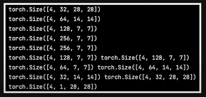
So you can see because we had downsampled only twice, our smallest size input to any convolution layer is 7x7. The code on the repository is much more configurable and creates these blocks based on whatever configuration is passed and can create multiple layers as well. We’ll look at a sample config file later, but first let’s take a brief look at the dataset, training and sampling code.
class MnistDataset(Dataset):
    r"""
    Nothing special here. Just a simple dataset class for mnist images.
    Created a dataset class rather using torchvision to allow
    replacement with any other image dataset
    """
    def __init__(self, split, im_path, im_ext='png'):
        r"""
        Init method for initializing the dataset properties
        :param split: train/test to locate the image files
        :param im_path: root folder of images
        :param im_ext: image extension. assumes all
        images would be this type.
        """
        self.split = split
        self.im_ext = im_ext
        self.images, self.labels = self.load_images(im_path)
The dataset class is very simple, it just takes in the path where the images are and then stores the filename of all those images in there.
def load_images(self, im_path):
    r"""
    Gets all images from the path specified
    and stacks them all up
    :param im_path:
    :return:
    """
    assert os.path.exists(im_path), "images path {} does not exist".format(im_path)
    ims = []
    labels = []
    for d_name in tqdm(os.listdir(im_path)):
        for fname in glob.glob(os.path.join(im_path, d_name, '*.{}'.format(self.im_ext))):
            ims.append(fname)
            labels.append(int(d_name))
    print('Found {} images for split {}'.format(len(ims), self.split))
    return ims, labels
Right now we are building unconditional diffusion model, so we don’t really use the labels.
def __len__(self):
    return len(self.images)

def __getitem__(self, index):
    im = Image.open(self.images[index])
    im_tensor = torchvision.transforms.ToTensor()(im)

    # Convert input to -1 to 1 range.
    im_tensor = (2 * im_tensor) - 1
    return im_tensor
Then we simply load the images and convert it to tensor and we also scale it from minus one to one, just like the authors, so that our model consistently sees similarly scaled images as compared to the random noise.
Code for Diffusion Model Training
Moving to train_DDPM.py, where the train() function loads up the config and
gets the model, dataset, diffusion and training configurations from it.
def train(args):
    # Read the config file #
    with open(args.config_path, 'r') as file:
        try:
            config = yaml.safe_load(file)
        except yaml.YAMLError as exc:
            print(exc)
    print(config)
    ########################

    diffusion_config = config['diffusion_params']
    dataset_config = config['dataset_params']
    model_config = config['model_params']
    train_config = config['train_params']

    # Create the noise scheduler
    scheduler = LinearNoiseScheduler(num_timesteps=diffusion_config['num_timesteps'],
                                     beta_start=diffusion_config['beta_start'],
                                     beta_end=diffusion_config['beta_end'])

    # Create the dataset
    mnist = MnistDataset('train', im_path=dataset_config['im_path'])
    mnist_loader = DataLoader(mnist, batch_size=train_config['batch_size'], shuffle=True, num_workers=4)

    # Instantiate the model
    model = Unet(model_config).to(device)
    model.train()

    # Create output directories
    if not os.path.exists(train_config['task_name']):
        os.mkdir(train_config['task_name'])

    # Load checkpoint if found
    if os.path.exists(os.path.join(train_config['task_name'],train_config['ckpt_name'])):
        print('Loading checkpoint as found one')
        model.load_state_dict(torch.load(os.path.join(train_config['task_name'],
                                                      train_config['ckpt_name']), map_location=device))
    # Specify training parameters
    num_epochs = train_config['num_epochs']
    optimizer = Adam(model.parameters(), lr=train_config['lr'])
    criterion = torch.nn.MSELoss()

    # Run training
    for epoch_idx in range(num_epochs):
        losses = []
        for im in tqdm(mnist_loader):
            optimizer.zero_grad()
            im = im.float().to(device)

            # Sample random noise
            noise = torch.randn_like(im).to(device)

            # Sample timestep
            t = torch.randint(0, diffusion_config['num_timesteps'], (im.shape[0],)).to(device)

            # Add noise to images according to timestep
            noisy_im = scheduler.add_noise(im, noise, t)
            noise_pred = model(noisy_im, t)

            loss = criterion(noise_pred, noise)
            losses.append(loss.item())
            loss.backward()
            optimizer.step()
        print('Finished epoch:{} | Loss : {:.4f}'.format(
            epoch_idx + 1,
            np.mean(losses),
        ))
        torch.save(model.state_dict(), os.path.join(train_config['task_name'],
                                                    train_config['ckpt_name']))

    print('Done Training ...')
We then instantiate the noise scheduler, dataset and our model. After setting up the optimizer and the loss functions, we run our training loop. Here we take our image batch, sample random noise of shape B x 1 x h x w, and sample random timesteps.
The scheduler adds noise to these batch images based on the sample timesteps, and we then backpropagate based on the loss between noise prediction by our model and the actual noise that we added.
Code for Sampling in Denoising Diffusion Probabilistic Model
For sampling, similar to training, we load the config and necessary parameters, our model and noise scheduler.
def infer(args):
    # Read the config file #
    with open(args.config_path, 'r') as file:
        try:
            config = yaml.safe_load(file)
        except yaml.YAMLError as exc:
            print(exc)
    print(config)
    ########################

    diffusion_config = config['diffusion_params']
    model_config = config['model_params']
    train_config = config['train_params']

    # Load model with checkpoint
    model = Unet(model_config).to(device)
    model.load_state_dict(torch.load(os.path.join(train_config['task_name'],
                                                  train_config['ckpt_name']), map_location=device))
    model.eval()

    # Create the noise scheduler
    scheduler = LinearNoiseScheduler(num_timesteps=diffusion_config['num_timesteps'],
                                     beta_start=diffusion_config['beta_start'],
                                     beta_end=diffusion_config['beta_end'])
    with torch.no_grad():
        sample(model, scheduler, train_config, model_config, diffusion_config)
The sample method then creates a random noise sample based on number of images requested and then we go through the timesteps in reverse.
def sample(model, scheduler, train_config, model_config, diffusion_config):
    r"""
    Sample stepwise by going backward one timestep at a time.
    We save the x0 predictions
    """
    xt = torch.randn((train_config['num_samples'],
                      model_config['im_channels'],
                      model_config['im_size'],
                      model_config['im_size'])).to(device)
    for i in tqdm(reversed(range(diffusion_config['num_timesteps']))):
        # Get prediction of noise
        noise_pred = model(xt, torch.as_tensor(i).unsqueeze(0).to(device))

        # Use scheduler to get x0 and xt-1
        xt, x0_pred = scheduler.sample_prev_timestep(xt, noise_pred, torch.as_tensor(i).to(device))

        # Save x0
        ims = torch.clamp(xt, -1., 1.).detach().cpu()
        ims = (ims + 1) / 2
        grid = make_grid(ims, nrow=train_config['num_grid_rows'])
        img = torchvision.transforms.ToPILImage()(grid)
        if not os.path.exists(os.path.join(train_config['task_name'], 'samples')):
            os.mkdir(os.path.join(train_config['task_name'], 'samples'))
        img.save(os.path.join(train_config['task_name'], 'samples', 'x0_{}.png'.format(i)))
        img.close()
For each timestep we get our model’s noise prediction and call the reverse process of scheduler that we had
created with this xt and noise prediction.
And then it returns the mean of xt-1 and estimate of the original image.
We can choose to either save or not these to see the progress of sampling.
Configurable Code
Now let’s also take a look at our config file.
dataset_params:
  im_path: 'data/train/images'

diffusion_params:
  num_timesteps : 1000
  beta_start : 0.0001
  beta_end : 0.02

model_params:
  im_channels : 1
  im_size : 28
  down_channels : [32, 64, 128, 256]
  mid_channels : [256, 256, 128]
  down_sample : [True, True, False]
  time_emb_dim : 128
  num_down_layers : 2
  num_mid_layers : 2
  num_up_layers : 2
  num_heads : 4

train_params:
  task_name: 'default'
  batch_size: 64
  num_epochs: 40
  num_samples : 100
  num_grid_rows : 10
  lr: 0.0001
  ckpt_name: 'ddpm_ckpt.pth'
This just has the dataset parameters, which stores our image path, model params, which stores parameters necessary to create model like the number of channels, down-channels and so on. Like I had mentioned, we can put in the number of layers required in each of our down-, mid- and up-blocks. And finally we specify the training parameters.
The Unet class in the repository has blocks, which actually read this config and create model based on whatever configuration is provided.
It does everything similar to what we just implemented, except that it loops over the number of layers as well.
And I’ve also added shapes of the output that we would get at each of those block calls so that it helps a bit in understanding everything.
Dataset for Training
For training, as I mentioned, I train on MNIST, but in order to see if everything works for RGB images, I also train on this dataset of texture images, because I already have it downloaded since my video on implementing DALL-E.
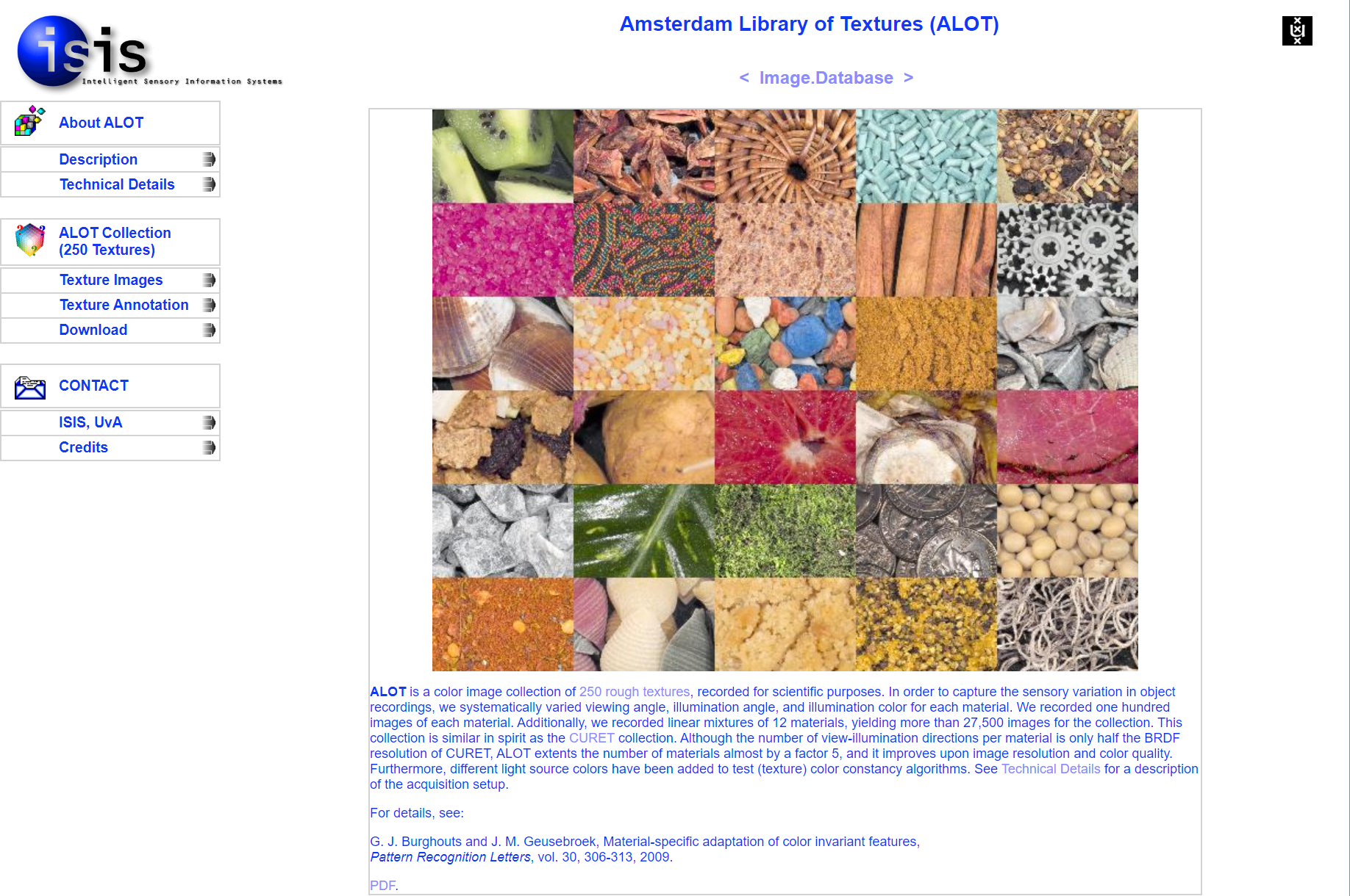
Here is a sample of images from this dataset. These are not generated, these are images from the dataset itself.
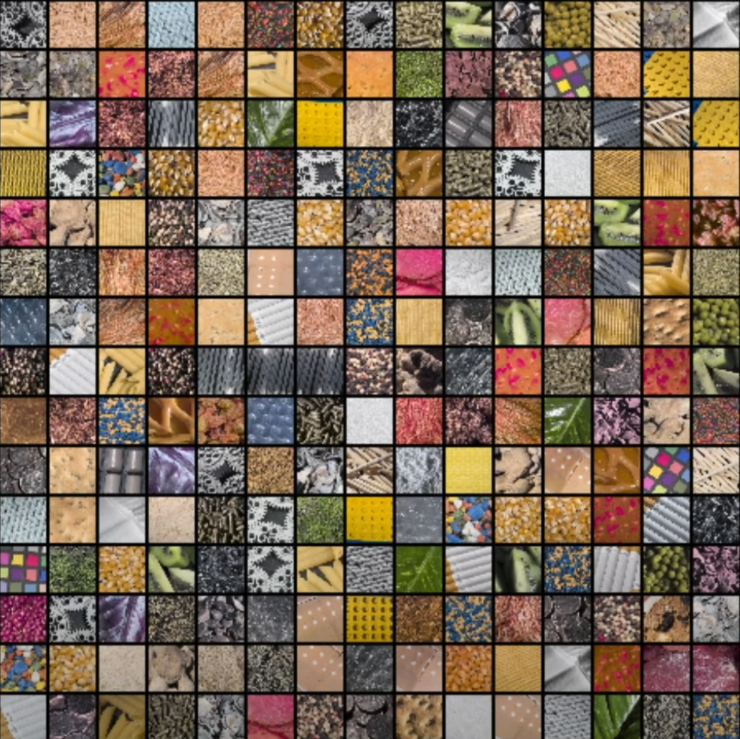
Though the dataset has 256x256 images, I resized the images to be 28x28, primarily because I lack two important things for training on larger sized images, patience and compute, rather cheap compute.
For MNIST I train it for about 20 epochs, taking 40 minutes on V100 GPU, and for this texture dataset I train for about 60 epochs taking roughly about 3 hours. And that gives me these results.
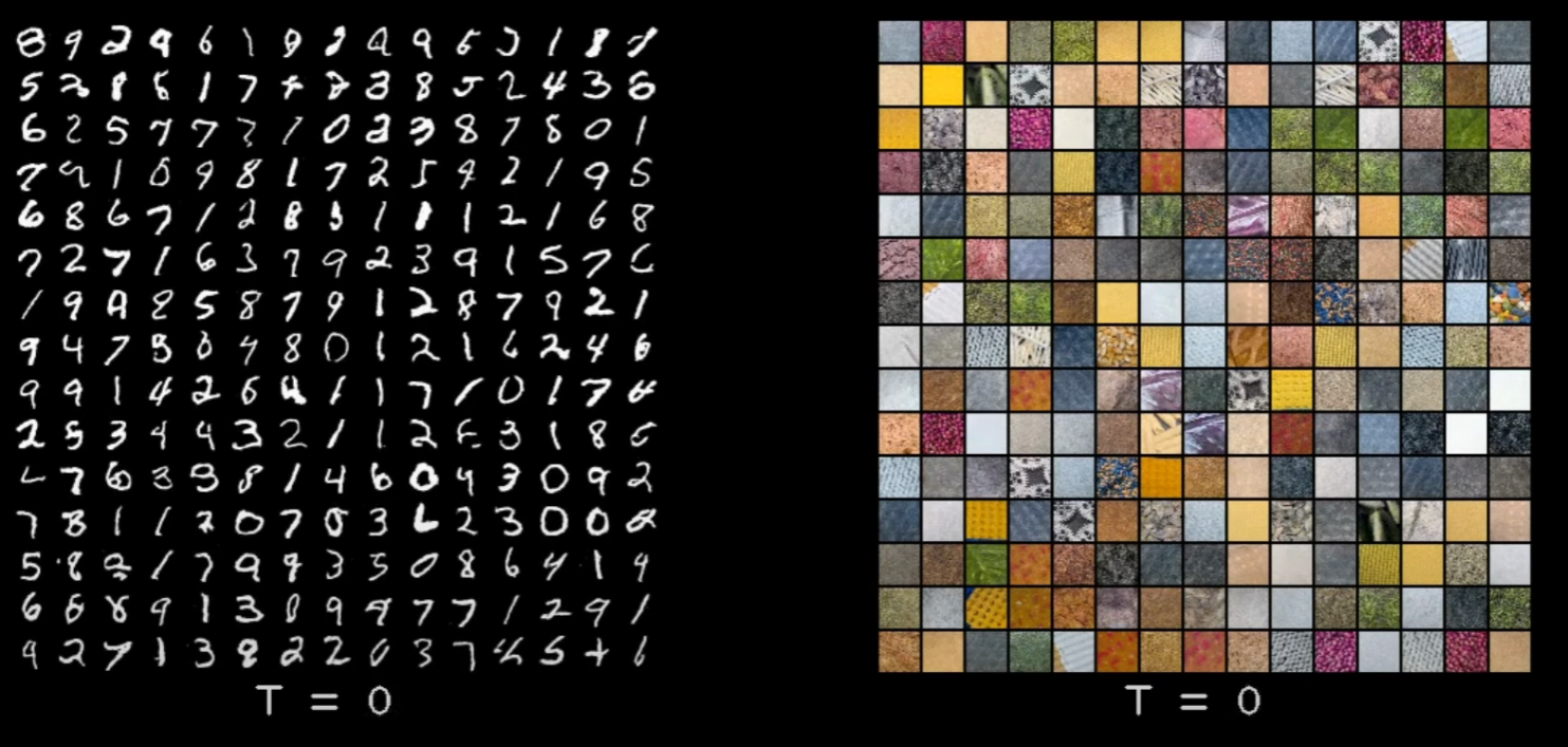
Results After DDPM Training
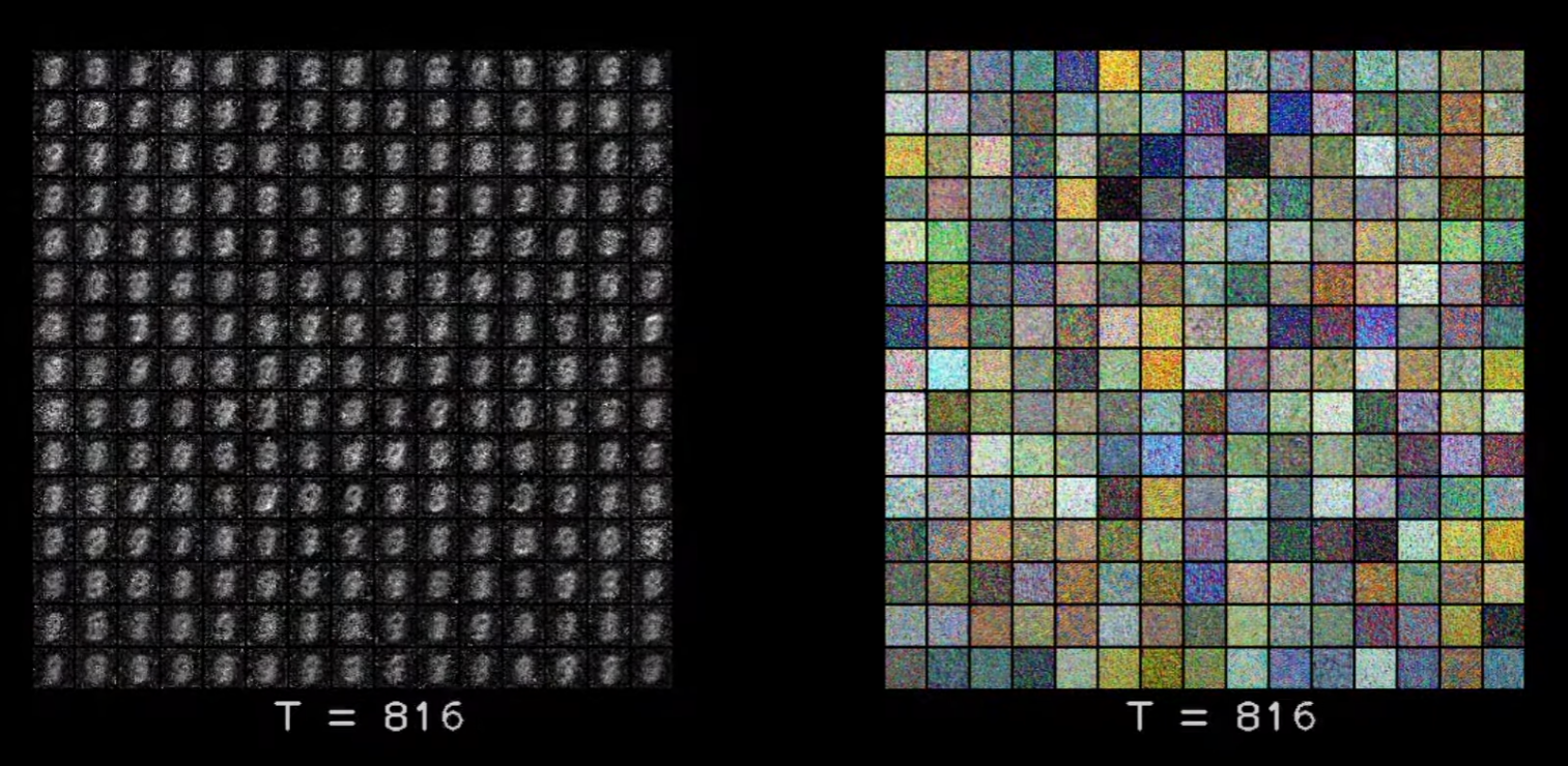
Here I am saving the original image prediction at each timestep. And you can see that because MNIST images are all similar looking, the model pretty quickly gets a decent original image prediction. Whereas for the textured data set it doesn’t till about last 200-300 timesteps. But by the end of all the steps we get decent results for both the data sets. You can obviously train it on a larger size data set, though probably you would have to maybe increase the channels, and maybe train for longer epochs to get nice results.
So that’s all that I wanted to cover for implementing DDPM. We went through scheduler implementation, unit implementation and saw how everything comes together in the training and sampling code. Hopefully it gave you a better understanding of diffusion models.
Thank You
And thank you so much for watching this video and if you are liking the content and getting benefit from it, do subscribe the channel. See you in the next video.


